(Original post: https://methodsblog.com/2019/08/21/thermal-images-r/)
1 Why use thermal images?
Temperature is important in ecology. Rising global temperatures have pushed ecologists and conservationists to better understand how temperature influences species’ risk of extinction under climate change. There’s been an increasing drive to measure temperature at the scale that individual organisms actually experience it. This is made possible by advances in technology.
Enter: the thermal camera. Unlike the tiny dataloggers that revolutionised thermal ecology in the past decade or so, thermal images capture surface temperature, not atmospheric temperature. Surface temperature may be as (if not more) relevant for organisms that are very small or flat, or thermoregulate via direct contact with the surface. Invertebrates and herps are two great examples of these types of organisms – and together make up a huge proportion of terrestrial biodiversity. Also, while dataloggers can achieve impressive temporal extent and resolution, they can’t easily capture temperature variation in space.
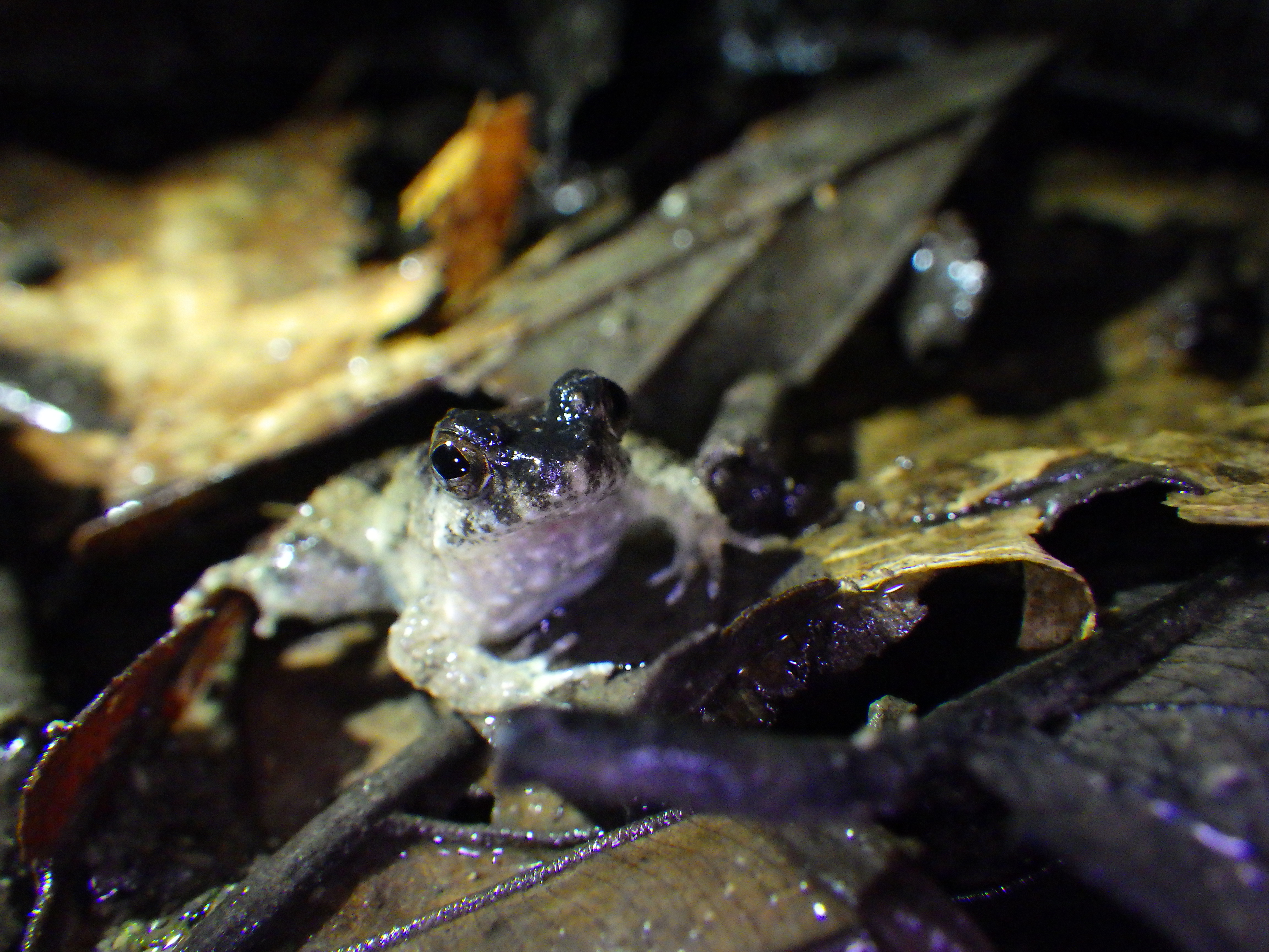
Surface temperature is important for small, flat things that don’t float in the air at breast height
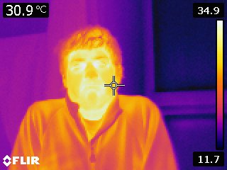
Like dataloggers, thermal cameras are becoming increasingly affordable and practical. The FLIR One smartphone attachment, for example, weighs in at 34.5 g and costs around ~US$300. For that, you get 4,800 spatially explicit temperature measurements at the click of a button. But without guidelines and tools, the eager thermal photographer runs the risk of accumulating thousands of images with no idea of what to do with them. So we created the R package ThermStats. This package simplifies the processing of data from FLIR thermal images and facilitates analyses of other gridded temperature data too.
2 What do I with all these images?
Too many images and no idea how to use them?
To start, it’s important to understand what a thermal camera actually measures. Each pixel in a FLIR thermal image has an embedded 16-bit value that represents the infrared radiation received by the sensor. What we want is the portion of that received radiation that was emitted by the object or scene of interest, because this is a function of its temperature.
2.1 Extracting the data
We need to convert the raw data to a temperature in °C using equations from infrared thermography (for information on how to extract this data, section 2.2 of ‘ThermStats: An R package for quantifying surface thermal heterogeneity in assessments of microclimates’). A few parameters are needed for this, including some that you should either measure or estimate:
- Emissivity = the amount of radiation emitted by a particular object, for a given temperature.
- Reflected apparent temperature = radiation that originates from other objects and is reflected by the object of interest.
- Object distance = the distance between the camera and the object of interest.
- Atmospheric temperature = the temperature of the atmosphere.
- Relative humidity = the relative humidity of the atmosphere.
The first two items on this list are difficult to measure in the field. Emissivity is likely to range between 0.92 (for dry, bare soil) and 0.99 (for green broadleaf forest). For high emissivities and short object distances, apparent temperature can be assumed to equal the atmospheric temperature.
2.2 Thermal metrics
We can calculate simple summary statistics at this point (mean, min, max etc.). But if that was all we wanted, we might as well use the trusty (and much cheaper) thermometer! The beauty of thermal images is their ability to capture temperature variation across space.
If we imagine that unique temperature values (at a given precision) are like species, we can use diversity indices to quantify thermal diversity. You might expect that more thermally diverse habitats would provide species with more opportunities for behavioural thermoregulation, for example. This has been suggested by some studies, but there remains much work to be done in this area.
We can also view a thermal image as a raster, akin to a land cover map. When we do this, clusters of pixels with a similar temperature are the equivalent of habitat patches. By borrowing techniques from landscape ecology – such as hot spot analysis – we can explore ideas like thermal connectivity and thermal fragmentation. This applies to thermal images and to coarser gridded temperature data.
There are two key functions for calculating thermal metrics. For a single thermal dataset, use get_stats, specifying your desired summary statistics and whether or not you want to (1) calculate connectivity and (2) identify hot and cold patches.
Alternatively, if you have multiple images within a specified grouping (e.g. one photo in each cardinal direction for multiple study plots; Senior et al. 2018; Scheffers et al. 2017), you can use stats_by_group. Many of the arguments are the same, but this function additionally allows you to define the grouping of the images.
By default, both get_stats and stats_by_group return a dataframe with patch statistics for each image or group, respectively.
2.3 Plotting
Both get_stats and stats_by_group can also return:
- the temperature dataset(s) in a dataframe format
SpatialPolygonsDataFrame(s) of hot and cold spots.
## Plotting distribution## Plotting image with hot and cold spots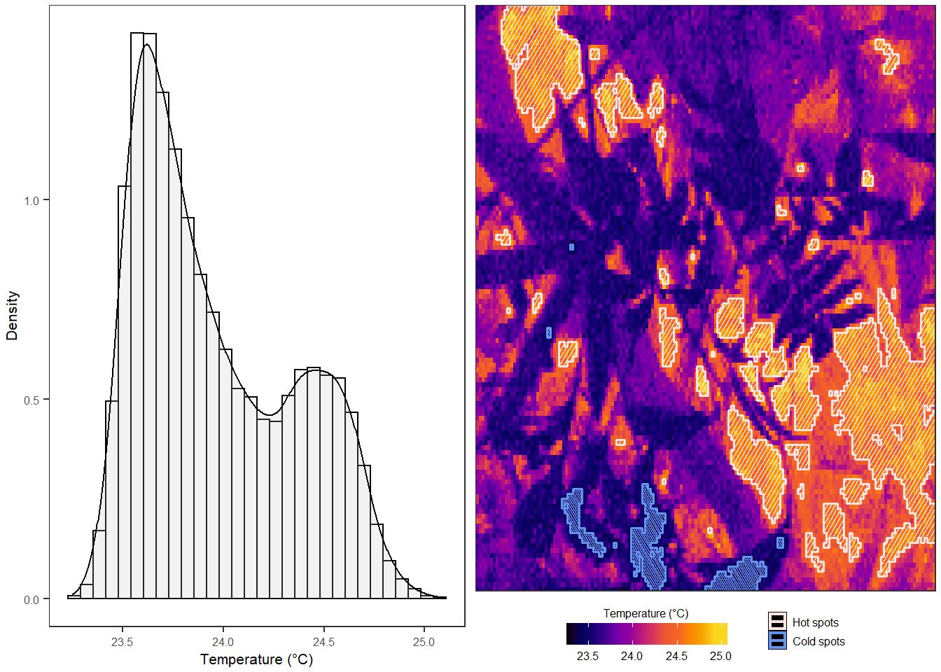
Figure 2.1: The output of plot_patches includes a histogram and the original temperature data overlaid with outlines of hot and cold spots, identified using the G* variant of the Getis-Ord local statistic.
The function plot_patches plots the temperature raster(s) overlaid with outlines of hot and cold spots, plus the temperature histogram if plot_distribution = TRUE.
A single temperature matrix can be converted to a RasterLayer using raster::raster(). A list of matrices (such as that returned by batch_convert) can be converted to a RasterStack using stack_imgs. Both RasterLayer and RasterStack objects can explored using the package rasterVis. Another option is to create violin plots of raster stacks using plot_stack, and consider the new package landscapemetrics for analysing and displaying hot and cold spots.
## Warning: multiple methods tables found for 'direction'## Warning: multiple methods tables found for 'gridDistance'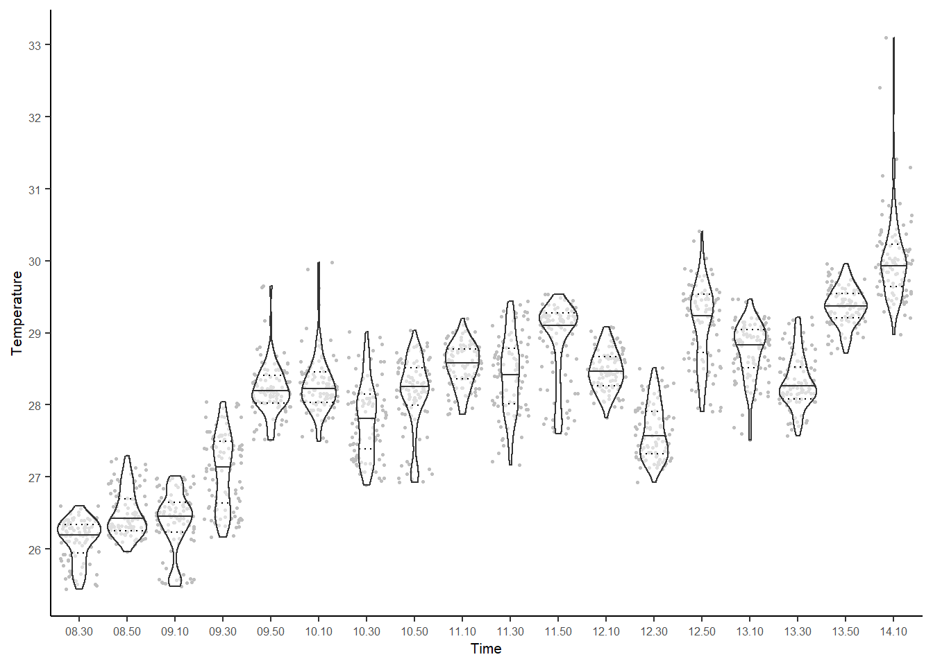
Figure 2.2: Violin plots created using plot_stack. Each datapoint is a single pixel, from the 100 pixels sampled at random from each raster. Rasters derive from thermal images collected every 20 minutes in the same location.
3 The Future
We welcome feedback and suggested enhancements, which you can submit as an issue to GitHub. I’d particularly like to implement processing of thermal images from other models of camera, but we currently only have access to FLIR images. Another obvious next step is testing out the biological relevance of our suggested thermal metrics. I’d be keen to hear from anyone who is interested in pursuing this!
A bright future for thermal ecology
To find out more about what you can do using ThermStats, read our Methods in Ecology and Evolution article ‘ThermStats: An R package for quantifying surface thermal heterogeneity in assessments of microclimates’
This is work I did as part of my PhD, with Prof David Edwards (University of Sheffield) and Prof Jane Hill (University of York). I was funded by ACCE (Adapting to the Challenges of a Changing Environment), which is a NERC (Natural Environment Research Council) Doctoral Training Partnership.